Fibroblast to neuron
[1]:
import phlower
import numpy as np
import pandas as pd
import networkx as nx
from itertools import chain
import scipy
import sklearn
import pydot
import seaborn as sns
import matplotlib.pyplot as plt
from scipy.stats import gaussian_kde
import scanpy as sc
from matplotlib.backends.backend_pdf import PdfPages
[2]:
%load_ext autoreload
%autoreload 2
import phlower
import importlib
importlib.reload(phlower)
phlower.__version__
[2]:
'0.1.3'
[3]:
adata = phlower.dataset.fib2neuro()
Downloading data to data/fib2neuro.h5ad
ddhodge to get embeddings and pseudo time
Parameters
basis: will perform PCA if set to None
root: start cell indecies for trajectory
k: bandwith for diffusion map affinity
npc: number of PCs to use
ndc: number of diffusion components to use
s: steps for diffusion process
lstsq_methods: least square methods for ddhodge potential calculation
[4]:
phlower.ext.ddhodge(adata, basis=None, roots=(adata.obs.group=="MEF"), k=7,npc=100,ndc=40,s=2, lstsq_method='cholesky', verbose=True)
Normalization:
done.
Pre-PCA:
2024-09-27 10:38:50.046613 distance_matrix
2024-09-27 10:38:50.085889 Diffusionmaps:
done.
2024-09-27 10:38:50.149426 diffusion distance:
2024-09-27 10:38:50.169049 transition matrix:
2024-09-27 10:38:50.174908 graph from A
2024-09-27 10:38:50.175141 Rewiring:
2024-09-27 10:38:50.175152 div(g_o)...
2024-09-27 10:38:50.350843 edge weight...
2024-09-27 10:38:50.390933 cholesky solve ax=b...
+ 1e-06 I is positive-definite
2024-09-27 10:38:50.396110 grad...
2024-09-27 10:38:50.509950 potential.
2024-09-27 10:38:50.592800 ddhodge done.
done.
2024-09-27 10:38:50.607937 calculate layouts
2024-09-27 10:38:58.920193 done
[5]:
figs = []
fig, ax = plt.subplots(1,1, figsize=(4, 3))
phlower.pl.nxdraw_group(adata,node_size=5, show_edges=False, label=False, ax=ax)

Delaunay triangulation to construct graph with holes
cluster_name: clusters to use, i.e. leiden or louvain
node_attr: pseudo time from ddhodge
start_n, end_n: how many cells to use to connect start and and clusters
circle_quant: quantile cells of each cluster to use for the starts ends connecting
calc_layout: if calculate layout using neato for the graph with holes
[6]:
phlower.tl.construct_delaunay(adata, cluster_name='group', node_attr='u', start_n=10, end_n=10, circle_quant=0.1, calc_layout=True)
start clusters ['MEF']
end clusters ['Neuron', 'Myocyte']
Now we can check the graph with holes and how pseudo time presents in the graph
[7]:
fig, ax = plt.subplots(1,2, figsize=(10, 3), constrained_layout=True)
phlower.pl.nxdraw_group(adata, graph_name="X_pca_ddhodge_g_triangulation_circle",node_size=5, show_edges=True, show_legend=True, label=False, ax=ax[0])
phlower.pl.nxdraw_score(adata, graph_name="X_pca_ddhodge_g_triangulation_circle",node_size=5, ax=ax[1], colorbar=True)

We can als check the graph with holes and the triangle distributions
[8]:
fig, ax = plt.subplots(1,2, figsize=(10, 3), constrained_layout=True)
phlower.pl.nxdraw_group(adata, graph_name='X_pca_ddhodge_g_triangulation_circle',layout_name='X_pca_ddhodge_g_triangulation_circle',node_size=5, show_edges=True, labelstyle='text',labelsize=8, show_legend=True, ax = ax[0])
phlower.pl.nxdraw_score(adata, graph_name='X_pca_ddhodge_g_triangulation_circle',layout_name='X_pca_ddhodge_g_triangulation_circle', colorbar=True,node_size=5, label=False, ax=ax[1])
fig, ax = plt.subplots(1,1, figsize=(5, 3))
phlower.pl.plot_triangle_density(adata, "X_pca_ddhodge_g_triangulation_circle", "X_pca_ddhodge_g_triangulation_circle", colorbar=True, edge_color='gray', ax = ax, node_size=5)


Graph holdge laplacian
In here, we first get normlized hodge laplacian and perform eigen decomposition to get the signals on edges
[9]:
phlower.tl.L1Norm_decomp(adata)
0.15503668785095215 sec
We can check the eigen vectors(harmonic) with eigen vectors = 0
[10]:
figs = []
fig, ax = plt.subplots(1,1, figsize=(5, 3))
phlower.pl.nxdraw_holes(adata, vector_dim=0,arrows=False, width=4, node_size=2, ax=ax, colorbar=True)
fig, ax = plt.subplots(1,1, figsize=(5, 3))
phlower.pl.nxdraw_holes(adata, vector_dim=1,arrows=False, width=4, node_size=2, ax=ax, colorbar=True)
fig, ax = plt.subplots(1,1, figsize=(4, 3))
phlower.pl.plot_eigen_line(adata, n_eig=8, linewidth='2', markersize=8, show_legend=False, ax=ax)


Check how many harmonic functions by checking 0 eigen values
[11]:
phlower.tl.knee_eigen(adata)
knee eigen value is 2
Preference random walk
[12]:
phlower.tl.random_climb_knn(adata, n=10000)
100%|██████████| 10000/10000 [00:04<00:00, 2116.66it/s]
[13]:
#G_ae.nodes(data=True)
from scipy import constants
fig_width = 9
fig, axs = plt.subplots(1, 2,figsize=(8, 3))
phlower.pl.plot_traj(adata, trajectory=adata.uns['knn_trajs'][0], colorid=0, node_size=1, ax=axs[0])
phlower.pl.plot_traj(adata, layout_name="X_pca_ddhodge_g_triangulation_circle", trajectory=adata.uns['knn_trajs'][0], colorid=0, node_size=1, ax=axs[1])

Project trajectories to harmonic space
[14]:
phlower.tl.trajs_matrix(adata)
2024-09-27 10:39:25.716062 projecting trajectories to simplics...
2024-09-27 10:39:32.647217 Embedding trajectory harmonics...
eigen_n < 1, use knee_eigen to find the number of eigen vectors to use: 2
eigen_n is 2, use itsself as embedding
2024-09-27 10:39:32.739772 done.
dbscan clustering on the culmulative trajectory space
[15]:
from collections import Counter
phlower.tl.trajs_clustering(adata, eps=0.5)
Counter(adata.uns['trajs_clusters'])
[15]:
Counter({0: 9276, 1: 724})
[16]:
c0 = np.where(adata.uns['trajs_clusters'] == 0)[0]
c1 = np.where(adata.uns['trajs_clusters'] == 1)[0]
plot clustered trajectories on the graph
[17]:
fig1, ax = plt.subplots(1,2, figsize=(8,3))
import colorcet as cc
color_palette = sns.color_palette(cc.glasbey, n_colors=50).as_hex()
phlower.pl.plot_traj(adata, layout_name="X_pca_ddhodge_g_triangulation_circle", trajectory=list(np.array(adata.uns['knn_trajs'], dtype=object)[c0[9]]), colorid=0, node_size=6, alpha_nodes=.8, ax=ax[0], edge_width=4,alpha=1, color_palette=color_palette, arrowsize=15)
def edges_on_path(path):
return zip(path, path[1:])
for a_traj in list(np.array(adata.uns['knn_trajs'], dtype=object)[c1[[2]]]):
nx.draw_networkx_edges(adata.uns['X_pca_ddhodge_g_triangulation_circle'],
adata.obsm['X_pca_ddhodge_g_triangulation_circle'],
ax=ax[0],
edgelist=list(edges_on_path(a_traj)),
node_size=10,
width=4,
edge_color=color_palette[1],
arrows=True,
arrowstyle='->',
arrowsize=5,
alpha=1
)
phlower.pl.plot_traj(adata, layout_name="X_pca_ddhodge_g", trajectory=list(np.array(adata.uns['knn_trajs'],dtype=object)[c0[9]]), colorid=0, node_size=6, alpha_nodes=.8, ax=ax[1], edge_width=4,alpha=1, color_palette=color_palette, arrowsize=15)
for a_traj in list(np.array(adata.uns['knn_trajs'],dtype=object)[c1[[2]]]):
nx.draw_networkx_edges(adata.uns['X_pca_ddhodge_g_triangulation_circle'],
adata.obsm['X_pca_ddhodge_g'],
ax=ax[1],
edgelist=list(edges_on_path(a_traj)),
node_size=10,
width=4,
edge_color=color_palette[1],
arrows=True,
arrowstyle='->',
arrowsize=5,
alpha=1
)

harmonic space for the two trajectory clusters
[18]:
import matplotlib
matplotlib.rc('xtick', labelsize=20)
matplotlib.rc('ytick', labelsize=20)
_, ax = plt.subplots(1,1, figsize=(4,3))
phlower.pl.plot_trajs_embedding(adata, clusters="trajs_clusters",show_legend=False, labelsize=40, node_size=10, ax=ax)

Create stream tree in harmonic space
trajs_use: how many trajectories to use
trajs_clusters: trajectory clusters
min_bin_number: Bin each trajectory group by pseudo time, the minimu bins for the shortest trajectory
cut_threshold: 1 by default, for the tree creating, in the harmonic space.
eigen_n: how many harmonic functions to use, default = -1 will use all.
[19]:
phlower.tl.harmonic_stream_tree(adata,
trajs_use=10000,
trajs_clusters='trajs_clusters',
min_bin_number=20,
cut_threshold=1,
layout_name='cumsum',
eigen_n=-1)
eigen_n < 1, use knee_eigen to find the number of eigen vectors to use
eigen_n: 2
{0, 1}
traj bins: 100%|██████████| 2/2 [00:11<00:00, 5.64s/it]
[(0, 1)]
edges projection: 100%|██████████| 10000/10000 [00:06<00:00, 1431.40it/s]
pseudo time bins for each trajectory group, and the tree created
Now we can plot the tree using STREAM
[20]:
celltype_colors = {
"MEF": "#0b871c",
"Neuron": "#fea541",
"d2_induced": "#d50a11",
"d2_intermediate": "#8b3df9",
"d5_earlyMyocyte":"#573b0a",
"d5_earlyiN":"#fe7fce",
"d5_failedReprog": "#6a034d",
"d5_intermediate":"#99fe40",
"d22_failedReprog":"#035659",
"Myocyte":"#573b0a",
}
adata.uns['group_color'] = celltype_colors
fig1 = phlower.ext.plot_stream_sc(adata, color=['group'], show_text=True, show_graph=True, show_legend=True, fig_size=(8,3), s=30, return_fig=True, dist_scale=.4)
fig2 = phlower.ext.plot_stream(adata, color=['group'], show_legend=True, fig_size=(8,3), return_fig=True, dist_scale=1)
None
{'S0': '1_21', 'S3': '2_21', 'S1': '0_17', 'S2': 'root'}


[ ]:
Trajectories in harmonic space, and culmulative harmonic space.
[21]:
figs = []
fig, ax = plt.subplots(1,2, figsize=(6,3), constrained_layout=True)
phlower.pl.plot_trajs_embedding(adata, clusters="trajs_clusters",show_legend=False, labelsize=40, node_size=10, ax=ax[0])
phlower.pl.plot_trajectory_harmonic_lines(adata, sample_ratio=0.05, show_legend=False, ax=ax[1])

[22]:
phlower.pl.plot_trajectory_harmonic_lines_3d(adata, sample_ratio=.1, show_legend=True, fig_path=None)
[23]:
phlower.pl.plot_trajectory_harmonic_points_3d(adata, sample_ratio=.1, show_legend=True, fig_path=None)
3
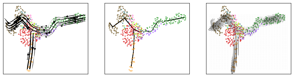
We also visualize the trajectories using velocity stream plots.
[24]:
figs = []
fig, ax = plt.subplots(1,3, figsize=(12, 3))
phlower.pl.fate_velocity_plot(adata, group_name='group',figtype='stream', ax=ax[0], show_legend=False, radius=100, maxlinewidth=10, embedd_label=False)
phlower.pl.fate_velocity_plot(adata, group_name='group',node_alpha=.5,figtype='point', ax=ax[1], show_legend=False, embedd_label=False)
phlower.pl.fate_velocity_plot(adata, group_name='group',node_alpha=.5,figtype='grid', ax=ax[2], show_legend=False, embedd_label=False, radius=100)
Leaf markers and transition markers
[25]:
import pickle
import os
from datetime import date
if not os.path.exists("save"):
os.mkdir('save')
today_ = date.today().strftime("%Y-%m-%d")
pickle.dump(adata, open(f"save/fib2neuron_{today_}.pickle", 'wb'))
[ ]: